
How to Make Your Interactive Digital Humans Fast#
When it comes to human-machine interaction, no matter how realistic the avatar looks and expresses, people expect instantaneous responses. A delay of even a few hundred milliseconds can make the digital human feel unresponsive or robotic. Unfortunately, with today’s technology, the pipeline from user speech to avatar response is long and complex, and it is tremendously challenging to make it fast enough to feel natural. In this post, I will explain the key factors that contribute to latency, and how to optimize them to achieve a fluid, real-time experience.
But the general direction is clear: we will restructure the pipeline with the following principles:
Streaming — emit each piece of output as soon as it is ready, rather than buffering the whole response.
Parallelization — don’t let stages sit idle. Overlap them wherever the dependencies allow.
The process of digital human Interaction#
We can recap the process of digital human interaction as a pipeline of stages.
The frontend captures user audio and streams it to an Automatic Speech Recognition (ASR) service. The transcript is passed to a cognitive engine, usually composed of Large Language Models (LLMs), which generates the textual response and associated behavioral context.
The text is converted to audio via Text-to-Speech (TTS). The audio then drives neural rendering: a pre-recorded image or video loop of the avatar is warped to match the speech, producing synchronized lip and facial motion. (Alternatively, diffusion-based synthesis, which generates every pixel from scratch, may remain too slow for real-time use.) We treat TTS and video generation as a single combined stage — the renderer.
The synchronized video and audio are combined and streamed back to the user for playback.
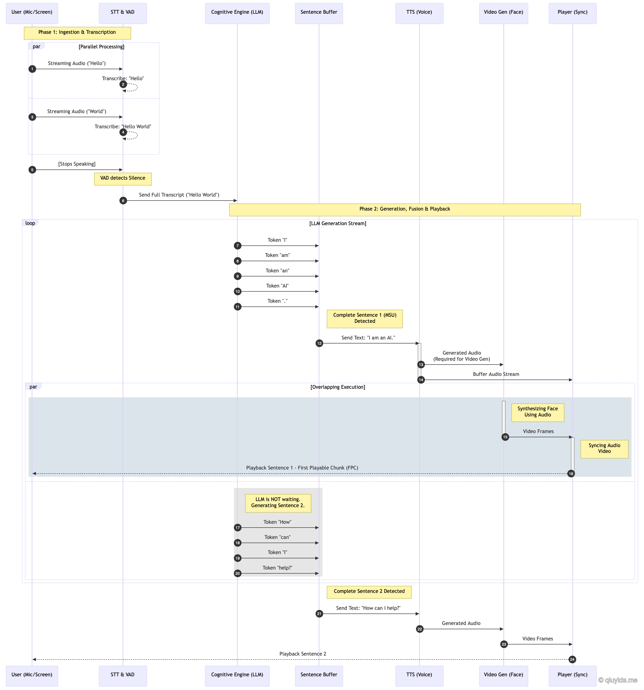
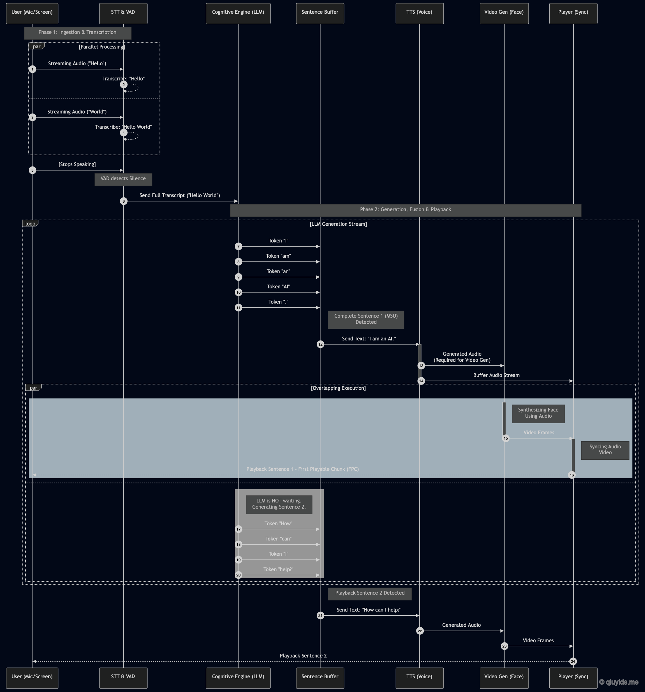
In a streaming pipeline these stages overlap rather than running sequentially:
ASR begins transcribing before the user has finished speaking, emitting partial transcripts in real time.
LLM receives the full transcript once ASR finalizes it, then immediately begins generating — streaming its output text to the renderer as they are produced.
Renderer starts processing the moment the first chunk of text is available, without waiting for the full LLM response to be generated.
Playback begins as soon as the first rendered frames and audio samples are ready, while upstream stages are still producing the rest of the response.
Latency Decomposed: Definitions and Measurements#
For the following subsections, we will build the timing model of the pipeline. The goal is to identify the bottlenecks and understand how to optimize them. We will define the key metrics, break down the latency into its components: starting with the Minimum Synthesis Unit (MSU), the atomic unit of pipeline work, then deriving First Response Time (FRT) and subsequent pipeline recurrence which allows us to understand the total completion time and fluidity of the pipeline.
Minimum Synthesis Unit (MSU)#
An MSU (Minimum Synthesis Unit) is the smallest chunk of output text that the synthesis stages can process into natural media — typically a sentence or a complete clause.
We cannot stream LLM output token by token to downstream stages: a TTS engine cannot intonate a single word, and the video stage needs an audio segment, not a phoneme, to animate the face. Instead, a sentence buffer accumulates generated texts from the LLM stream and cuts at MSU boundaries; In the output streaming pipeline, every downstream stage — synthesis, transmission, playback — operates MSU by MSU.
First Response Time (FRT)#
The First Response Time (FRT) is the interval from end-of-speech to the first frame of synchronized media playing on the device:
Where:
\(D_{ASR}\): speech recognition — \(D_{VAD}\) (voice activity detection) plus \(D_{STT}\) (speech-to-text).
\(D_{Ingress}\): one-time network latency to send the user’s input in.
\(d_{Egress}(i)\): network latency to stream MSU \(i\)’s media back to the frontend.
\(d_{LLM}(i)\): time for the LLM to generate MSU \(i\), including queue delay.
\(d_{Render}(i)\): time for the renderer to produce media for MSU \(i\), including queue delay.
For short responses (1–2 MSUs) the startup cost dominates; for long ones, per-MSU throughput dominates.
Pipeline Recurrence#
This section models how the pipeline progresses MSU by MSU, which shows the interdependence of components.
Once the first MSU is released, the pipeline runs as a loop:
The LLM keeps generating tokens. A sentence buffer accumulates them, and whenever the buffered text hits an MSU boundary, that MSU is released to the renderer.
A released MSU starts rendering as soon as a worker is free — the input text exists and the resource is available.
The frontend plays finished MSUs in order: each one starts when it has arrived and the previous one has finished playing.
Let \(L_i\) be the time the LLM finishes writing MSU \(i\), \(R_i\) the time media synthesis finishes for it, and \(A_i\) the time MSU \(i\) arrives at the frontend. \(L_i\) and \(R_i\) are elapsed times measured from the moment the backend receives the completed user turn — hence \(L_0 = R_0 = 0\). \(A_i\) is on the user’s clock, so its formula first shifts the origin back to end-of-speech by adding the input-side costs \(D_{ASR} + D_{Ingress}\):
Effectively, the renderer starts rendering when text is ready, the worker is free, and — when frame-dependent — the previous MSU’s last frame is available. With one worker the latter two coincide, so the recurrence uses \(R_{i-1}\) for both.
LLM Part#
Every LLM inference request passes through three phases:
Request overhead. The one-time cost to initiate an inference request — network round-trip, API gateway overhead, and request dispatch. Denoted \(D_{Overhead}\). Load-dependent waiting is tracked separately as queue delay.
Prefill. The model processes the entire input in parallel over all input tokens. Paid once per request. Denoted \(D_{Prefill}\).
Decode. The model emits tokens one by one. Decode is sequential; denote the steady-state output rate \(\mathrm{TPS}\) (tokens per second), so \(k\) tokens cost \(k/\mathrm{TPS}\).
Request overhead and prefill are fixed one-time costs paid at the start of inference. Decode is the only variable, per-MSU cost — it runs continuously across the response, with the sentence buffer cutting the token stream into MSU boundaries. The service time is a fixed part plus a variable part:
where \(T_i\) is the token count of MSU \(i\), and \(\mathbf{1}_{i=1}\) is 1 for the first MSU and 0 otherwise. The fixed costs land entirely on MSU 1; every subsequent MSU pays only decode cost.
For the first MSU, we often denote the fixed startup cost as time to first token (TTFT) — the elapsed time from request submission to the first generated token from consumer point of view.
Rendering part#
The renderer combines TTS and video synthesis into a single stage. \(d_{Render}(i)\) includes:
TTS. Converts text to audio for MSU \(i\).
Video. Warps the avatar to match the generated audio.
In practice, rendering is the heavier stage: \(d_{Render}(i)\) typically dominates \(d_{LLM}(i)\) for all but the largest models.
Whether rendering MSU \(i\) depends on the output of MSU \(i-1\) varies by technique:
Frame-dependent (sequential). The avatar’s last frame of MSU \(i-1\) is the starting visual state for MSU \(i\). The renderer must finish the previous MSU before starting the next. With one worker, the resource constraint and the data dependency point to the same timestamp (\(R_{i-1}\)), so the recurrence form is unchanged. The practical consequence is that extra workers cannot parallelize frame-dependent MSUs: each MSU chains on the last frame of its predecessor.
Frame-independent. Each MSU renders as a self-contained clip — the avatar resets to a neutral pose, or the clip is a standalone motion. Here \(R_{i-1}\) in the recurrence is purely a resource constraint (the single worker is busy). Extra workers can process independent MSUs in parallel, provided the LLM is not the bottleneck.
We here assume one render worker per allocated rendering resource — that is, the renderer processes MSUs sequentially on a dedicated worker. A physical GPU can be scheduled to run multiple jobs concurrently, but each additional job contends for memory bandwidth and compute: throughput rises but per-job latency degrades. If a physical resource is partitioned into multiple worker nodes, here the model assumes you reserve one entire worker node (with its fixed share of resources) for the full session, which is to assume the renderer is immediately available when the next MSU is ready — standard for latency-sensitive pipelines.
The recurrence \(R_i = \max(R_{i-1}, L_i) + d_{Render}(i)\) is natively compatible with the frame-dependent case: \(R_{i-1}\) is exactly when the last frame becomes available, so the data dependency is already encoded. In the frame-independent case the same recurrence holds only under the one-worker assumption — \(R_{i-1}\) then acts as a resource constraint, and the equation would need a different form with multiple workers.
To see which stage limits the pipeline, subtract consecutive terms of the recurrence:
Each term has a distinct meaning:
\(d_{Render}(i)\) — the time the renderer spends on actual work for this MSU.
\(\max(0, L_i - R_{i-1})\) — idle time: the renderer is free but waiting for the LLM to finish writing MSU \(i\).
When the LLM finishes before the renderer (\(L_i \leq R_{i-1}\)), the max term vanishes — LLM work is hidden under rendering, and the renderer is the bottleneck. When the LLM finishes late (\(L_i > R_{i-1}\)), the renderer stalls, and the LLM is the bottleneck. With one worker, the \(R_{i-1}\) in the condition serves as both a resource constraint (the worker is busy) and — when rendering is frame-dependent — a data dependency (MSU \(i\) needs the last frame of MSU \(i-1\)). Both resolve to the same timestamp under the one-worker assumption, so the recurrence form is unchanged. The distinction matters when you consider adding workers: frame-dependent MSUs cannot be parallelized even with spare capacity.
Total Completion Time#
The recurrence above produces \(R_N\) — the time the last of \(N\) MSUs finishes rendering. The last MSU reaches the frontend at:
This is when the final media chunk reaches the frontend, but the user finishes hearing it later. With \(S_N\) defined below, the playback completion time is \(T_{playback}=S_N+P_N\). \(T_{ready}\) is rarely the optimization target; FRT and fluidity matter more. The value of the closed form below is that it makes the bottleneck explicit.
Constant-cost simplification. Let \(l=\bar{d}_{LLM,>1}\) be the steady-state LLM cost for MSUs after the first, and let \(r=\bar{d}_{Render}\) be the typical media-synthesis cost. When later MSUs have roughly equal costs, the recurrence collapses to:
The first term includes TTFT, while the remaining terms describe steady-state production. If \(l\leq r\), media synthesis is the bottleneck; if \(l>r\), LLM decoding is the bottleneck. This approximation assumes similarly sized MSUs. For uneven responses, use the full recurrence instead: a large \(d_{LLM}(i)\) stalls the renderer; a large \(d_{Render}(i)\) creates a backlog that hides later LLM work.
Note that \(T_{ready}\) and \(T_{playback}\) measure different things: all media can be produced quickly (\(T_{ready}\) is low) while the user still hears gaps because an early MSU arrived late. A system optimized for completion is not necessarily fluid — the two goals must be tracked separately.
Fluidity#
Let \(P_i\) be the playback duration of MSU \(i\) and \(S_i\) the time it starts playing. Without an initial playback buffer, \(S_1=A_1\); thereafter, ordered playback gives
Fluidity is the absence of gaps between MSUs. Substituting the playback recursion, the gap before MSU \(i\) is
— how much MSU \(i\)’s arrival overshoots the end of MSU \(i-1\)’s playback; while positive, the avatar freezes on the last frame. Three rearrangements turn this into production terms — unwrap the max and move \(A_{i-1}\) to the right-hand side, difference the arrival equation (the input-side constants \(D_{ASR} + D_{Ingress}\) cancel), and expand \(R_i - R_{i-1}\) with the render recurrence:
Substituting the last two lines into the first gives the general condition:
When MSU \(i-1\) began playing on arrival (\(S_{i-1}=A_{i-1}\) — true right after a previous gap, or with no playback buffer), the slack term vanishes and the window reduces to \(P_{i-1}\) alone. This zero-slack form is conservative: any buffered slack only widens the window, so it never under-predicts a gap.
Two common causes, one for each side of the inequality:
Chunk-size mismatch. A short MSU shrinks the window \(P_{i-1}\) while a long one raises the production time \(d_{Render}(i)\) — the two sides move against each other.
Queue delays. Contention inflates the production time: \(d_{Render}(i)\) directly, or \(L_i\) through delayed LLM output. A pipeline fluid at idle can stutter under load.
Parallelism, Rendering Resources, and Playback Rate#
Throughout this article we assume one renderer per session. Production deployments usually share a pool of renderers across sessions, which introduces two complications into the analysis: random render queue time and fluctuating render speed from shared compute. I would argue that to fullfill the promise of fluidity, any single session must have at least one available renderer at any given time. To ensure that, a dedicated renderer per session is the simplest and a reasonable solution while extra wokers provide little benefit when production is already faster than consumption.
Production must outpace consumption. Playback is sequential. A single renderer typically produces media faster than the user consumes it, so overlapping the LLM writing MSU \(i+1\) while the renderer synthesizes MSU \(i\) is usually enough to keep the playback buffer full. When production cannot keep up, hiccups are unavoidable: the pipeline must supply each MSU before the user finishes the previous one. For stable MSUs in the single-renderer model, the practical target is
where \(p\) is the average playback duration of an MSU (the constant-cost equivalent of \(P_i\)). Leave headroom for variable sentence lengths, network jitter, and queue delays. If average production is slower than playback, any fixed buffer eventually drains. This is the single constraint that matters most for fluidity.
Extra workers help only when two conditions hold: MSUs render independently (no visual state carried from one to the next), and rendering, not the LLM, is the bottleneck (i.e., \(r > l\)). When both hold, extra workers reduce total completion time and prevent downstream gaps. When the LLM is the bottleneck (\(l \geq r\)), however, extra capacity buys nothing. Co-locating render jobs on the same GPU also contends for memory bandwidth and compute, slowing each job.
Key Takeaways#
If you find the above derivations bored, here are the key takeaways:
FRT and fluidity matter more than total completion time. A low \(T_{ready}\) does not guarantee a smooth experience — what the user feels is how quickly the avatar starts speaking, and whether it does so without interruption.
Production must outpace consumption. Every MSU must arrive before the previous one finishes playing. Buffers delay a stall; they never prevent one. The hard constraint is \(\max(l, r) \leq p\).
One renderer per session is the right baseline — it guarantees availability and makes the timing model tractable. Extra workers add little once production already outpaces consumption, and help only when MSUs are frame-independent and rendering is the bottleneck. When the LLM is the bottleneck, extra capacity sits idle.
What to do …#
Here are some practical techniques to reduce latency and improve fluidity.
Streaming Support#
The key to low latency is to allow output streaming, which the entire blog post is based on. And by far this perhaps is the most challenging part of the optimisation. There is a lot to iron out during the implementation, because it often involves lots of engineering work to do to make sure the streaming is smooth and stable. I would suggest that you should incorporate streaming support from the beginning of the project, if latency is a concern, because refactoring a non-streaming pipeline to a streaming one is often more expensive than building it from scratch.
Tracing#
Tracing is when you consolidate timing events from every stage, stamp them with a common trace ID, and assemble a single timeline per round. It is essential when stages are streamed across multiple machines — the frontend, your server, and remote APIs each see only their own slice. Traditional logging is hard to work with because it records events in isolation. That timeline reveals which stage is the bottleneck.
Record start and end times for every task. Overhead often hides inside a task, not between them. A task that looks fast alone may spend half its time in serialization or data conversion before the real work begins. Without both timestamps you see only the footprint, not where the time went. Network time in particular is invisible unless you record send timestamps on one side and receive timestamps on the other — the gap between them is your cross-machine hop.
Address VAD threshold#
Unfortunately the frontend replies on a length of silence to determine when the user has finished speaking, which introduces a latency that is often hard to reduce. The VAD endpointing defines a threshold for the length of silence that is considered as the end of the user turn. The longer the silence, the more confident the system is that the user has finished speaking, but it also adds latency to the response. While the input is streamed to backend, we could implement a two-stage endpointing to reduce the latency, where we apply a soft threshold and a hard threshold to the streamed input:
A soft threshold — short silence, fires quickly. The pipeline begins reversible work (ASR finalization, LLM prefill, first-token generation).
A hard threshold — longer silence, confirms the user has finished. The answer is committed and egress begins.
If speech resumes between the two, cancel the in-flight work and restart. This is branch prediction for voice: speculatively execute on the likely outcome, flush on a mispredict. Obviously the price we have to pay in this case is that we will need to waste some computation when the user resumes speaking.
Prompt Caching (KV Cache)#
Recall that \(D_{Prefill}\) is paid on every request. For a digital human, the prompt comprises static components: system instructions, persona, tool definitions, and few-shot examples do not change between turns. Most LLM services offer prompt caching (KV-cache reuse, prefix caching). If the model sees the same prefix of tokens across requests, it reuses the computed key-value activations from the first pass, skipping prefill for that prefix on subsequent calls. The win is big for agentic digital humans, where the system prompt is large and repetitive and each user turn is small, you not only save time but also save token costs.
Two things make this work in practice:
Organize the prompt for prefix stability. Place all static content at the front — system message, persona, tool schemas, shared RAG context — and only the conversation history and latest user turn at the end. The cache matches on strict prefix:
[static prefix | dynamic suffix]. A single shifted token at the front invalidates the entire cache.Mind the cache TTL. Prompt caches have a valid time — if you expect your app to receive requests after the TTL expires, the cache will become cold and you pay full prefill again. You may need to enable caching explicitly or extend the TTL to match your request frequency. Some services charge a storage premium for cached tokens.
Media Caching#
Media caching operates on the output side: when the LLM produces the same MSU text as a previous turn, skip TTS and video rendering and replay the cached media. This works when MSUs are frame-independent — the rendered output depends only on its own text, with no visual state carried from prior MSUs, so a cached clip can be dropped into any position in the output stream. When rendering is frame-dependent (the avatar’s expression carries across MSU boundaries), a cached clip may not blend seamlessly with the surrounding rendered MSUs; pre-render common phrases with neutral lead-in and lead-out frames, or restrict caching to the first MSU where no prior visual state exists. Greetings, confirmations, disclaimers, and standard prompts remain natural candidates for either approach.
Measure cache hit rate and hit-path FRT separately from the generative path. A high hit rate can conceal a slow renderer; keep the two paths independently monitored so you notice degradation before the cache expires.
Response Caching#
Response caching operates on the input side: when a user asks a question similar to one already answered, reuse the cached response text — and its pre-rendered media, if available — rather than invoking the LLM and renderer.
Semantic caching matches queries by meaning, not exact string. Two differently worded questions that ask the same thing hit the same cache entry. The win is substantial: a semantic hit skips the entire pipeline.
The risk is staleness. Cache only what is safe to reuse:
Static knowledge — FAQs, product details, definitions — can be cached aggressively with long TTLs.
Time-sensitive queries — weather, stock prices, news, “what’s on today” — must exclude from the cache or carry a short TTL with a data-version key tied to the freshness window. You may leverage the intent detector to classify queries into static vs. dynamic buckets, and apply different caching policies to each.
You may need to measure semantic-match precision alongside latency because the cost of such optimization is a small risk of returning a cached answer that is not actually correct for the current query.
Network Time#
Recall that \(D_{Overhead}\) includes a network round-trip — often the dominant one-time cost on the MSU 1 critical path, alongside \(D_{Prefill}\).
Co-locate services. Place the LLM API in the same cloud region as your renderer, and as close to the end user as possible. A user in Tokyo hitting a server in Virginia pays the round-trip on every turn. If you self-host, run services in the same cluster to eliminate the network hop entirely. The co-location benefit applies to every downstream stage, not just the LLM. Finding the right topology takes trial deployments — measure FRT from each candidate region and pick the one that minimizes the end-to-end hop.
Data Conversion Overhead#
Converting between formats on the hot path — numpy arrays to PyTorch tensors, text to token IDs, float32 to float16 — adds up when repeated per request.
Load in the target format. If your pipeline ends in PyTorch, load data with a torch-native loader rather than going through numpy. Where possible, load directly onto the GPU to skip the CPU to GPU transfer.
Store data contiguously. Contiguous memory layouts make downstream copies cheap and predictable. For hot-path tensors, ensure they are stored contiguously — it is a one-time cost that simplifies every operation that follows.
Pick a Fast-Enough LLM#
Recall that:
When the LLM is consistently faster than the renderer (\(l \leq r\)), the max term vanishes after the first MSU — the renderer never stalls waiting for text. The pipeline simplifies to \(R_N \approx d_{LLM}(1)+Nr\), with the renderer as the sole bottleneck. Gaps come only from uneven rendering cost, not from LLM jitter — one variable to debug instead of two.
The practical takeaway is that you do not need the largest, smartest model. Pick the fastest model that meets your quality bar. A 13B model that runs at 2× real-time buys more pipeline headroom than a 70B model that barely keeps up, and costs less to operate. Of course, the param size is not the only factor that determines the speed of the model, and you should benchmark the actual model while understanding the trade-offs between speed and quality.
Also pick a well-provisioned model. Models with broad adoption run on large, replicated fleets that absorb spikes. A niche or self-hosted model on a small GPU pool risks queueing under load.
Rendering Resolution#
\(d_{Render}(i)\) scales with output resolution. If your end user is on a phone, a 720p avatar already exceeds what the eye can resolve, pushing higher resolution adds cost with no perceptual gain. Detect the viewport at session start and select the resolution accordingly: lower latency for mobile, higher fidelity for desktop. Same principle as picking a fast-enough LLM: don’t pay for quality your users cannot perceive.
MSU Splitting in Sentence Buffer#
The sentence buffer sits between the LLM and the renderer. It watches the token stream, waits for a complete sentence or clause, and then releases that chunk as an MSU. The point is to cut early — the moment an MSU is ready, the renderer can start, and the pipeline stays busy.
Prompt the LLM. The simplest approach: tell the model to insert a boundary marker after each complete clause. The marker means “release this MSU now,” not “stop generating.” This costs a few prompt tokens and lets the model decide where the natural breaks fall, which almost always beats punctuation heuristics.
Sentence splitter (fallback). When you cannot prompt the LLM, fall back to splitting on sentence-ending punctuation. Set a minimum size so you do not ship "Hi." as its own MSU, and a maximum cap to break up long sentences — you trade a small intonation hit for keeping the pipeline fed. Tune these limits against measured \(P_i\), not token counts. LLM-supplied breaks take priority; the splitter is there for whatever the model misses.
Query Decomposition#
Users often pack multiple questions into a single turn: “What’s the fastest route to the airport, and how much is the fare?” These are two independent queries that the LLM can process in parallel rather than sequentially.
This decomposition typically happens at the intent-detection stage. When the classifier identifies multiple intents whose answers do not depend on each other, fork them into separate LLM calls. The downstream pipeline still needs the first answer first — the initial MSU is on the critical path — but the second query runs concurrently, so its latency is partially or fully hidden behind the first.
The constraint is independence. If query B needs the output of query A (“find me a hotel near the restaurant you just recommended”), they cannot be split; sequential is the only option. Check dependencies at the routing layer before forking.
Frontend-Side Slack#
MSU arrival times have variance — network jitter, variable decoding, uneven rendering. Two frontend-only techniques absorb it without touching the pipeline.
Playback buffer. The frontend holds back playback until \(B\) seconds of media have arrived, then starts playing. If a later MSU runs late, the buffer drains to cover the gap; when the pipeline recovers, the buffer refills. The trade-off is simple: you add \(B\) to FRT in exchange for absorbing jitter. Size \(B\) to cover pipeline variance — any larger and you are just adding latency with no further benefit.
Inter-MSU silence. Insert a brief silence between successive MSUs during playback. Natural speech already pauses at sentence boundaries; an additional 200ms is imperceptible but gives the pipeline a recurring window to catch up. A 100ms gap across six MSUs nets 500ms of slack — distributed across the utterance rather than concentrated at the start.
Both methods can operate purely at the frontend.
Hardware Scaling#
A common mistake is to reach for horizontal scaling (more GPUs) when vertical scaling (a faster GPU) is the right answer for a single session. Splitting one session’s rendering across two GPUs rarely helps: if the renderer is frame-dependent, MSUs must execute sequentially regardless of how many devices are available. Adding a second GPU introduces cross-device communication overhead — transferring the last frame, audio context, and avatar state between devices — that can make the combined setup slower than one faster GPU. One better GPU beats two cheaper ones for per-session latency.
Horizontal scaling is for multi-session throughput, not single-session speed. Scale the stage whose traces show the largest queue component, not the stage with the most impressive isolated benchmark. For the LLM, batch or replicate decode capacity only after checking TTFT and per-MSU P95 under the target concurrency. For media synthesis, add workers only when MSUs are frame-independent and \(\mathrm{RTF}_{Render}\) is near or above 1, or when \(d_{Render}^{queue}\) is material — otherwise a single faster render worker per session is the better investment.
Keep session affinity where visual state, voice state, or cache locality requires it. Autoscaling on GPU utilization alone reacts too late and cannot distinguish useful work from queueing; use queue depth, P95 queue time, and the fluidity error rate (\(G_i>0\)) as scaling signals.
Preloading#
Load everything the renderer needs into RAM once at session start. Convert the base avatar video to tensors, load the voice model weights, and read lookup tables from disk before the first user turn begins. These are one-time costs that should never appear inside \(d_{Render}(i)\).
The pattern is the same across asset types: pay the I/O and format conversion upfront, keep the result in GPU or CPU memory, and reuse it for every MSU. A base video that is re-decoded from disk per MSU adds a fixed-per-MSU I/O tax that looks like a slow renderer in traces.
Eager Egress#
You do not need to wait for the entire MSU to finish rendering before starting egress. The renderer produces frames sequentially; stream each one as it lands rather than buffering the full clip. For the first MSU, this cuts FRT by up to \(d_{Render}(1)\) — the first frame reaches the user while the renderer is still producing the rest of the MSU.
The trade is risk of a mid-MSU gap. If rendering slows or the network jitters mid-stream, the playback buffer drains and the user sees a stall — not between sentences, but inside one. Eager egress is worth it for the first MSU where FRT is the primary metric; for later MSUs the pipeline should already be ahead of playback, so the gain is marginal and the risk of gap is not justified.
Default Messages#
For common greetings, out-of-scope requests, and known error states, return a pre-approved default response with pre-rendered media. This removes the LLM and media-synthesis terms from the critical path, leaving only routing and egress. It is appropriate only when the response is semantically safe for the detected intent; do not use a cached default as a substitute for answering a specific question.
Track default-response rate and its FRT separately. A low average FRT obtained by serving many defaults is not evidence that the generative path meets its SLO.
Filler & Status Feedback#
If the LLM cannot produce the first MSU within the FRT target, fill the gap with a canned acknowledgement. A short phrase (“Let me look that up…”) with pre-recorded media buys decode time for the first substantive MSU at zero synthesis cost.
A related technique is the status update — a brief indication of progress mid-turn (“Searching your files…”, “Checking availability…”) when a backend operation runs long. Unlike a filler, which buys time for the LLM, a status update buys time for an external action the user asked for. It signals that work is in progress and prevents the user from repeating their request.
Both techniques work on the same principle: not all silence weights the same. Silence before the first response is the heaviest — the user has no signal that the system is alive. Silence after an acknowledgement is lighter: the user knows work is underway. Inter-MSU silence at sentence boundaries is the lightest — it mirrors natural speech prosody and is rarely noticed. A 500ms gap before any response feels broken; the same 500ms between sentences feels normal. Use fillers and status updates to shift silence from the heavy category to the light one — you are not reducing latency, you are reducing the perceived weight of the latency that remains.